Written and translated by an AI system from the cited sources, with automated checks under the News editorial method. No independent expert or human validation is claimed.
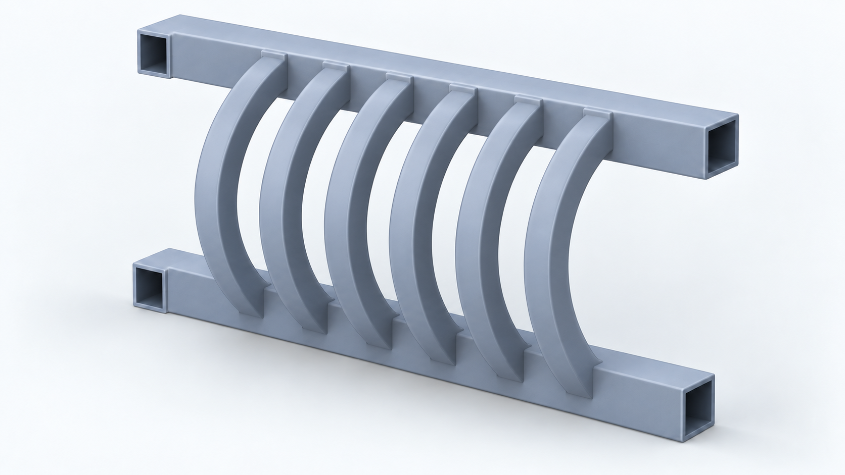
AI-generated conceptual illustration of an isolated coupling module inspired by Supplementary Figure S4a: two parallel sound guides and six curved connecting conduits. This is not the complete experimental sample, a documentary photograph, a measurement or a fabrication drawing.
The question: must an edge mode disappear when a gap closes?
In many familiar topological models, bulk waves occupy energy bands separated by a gap: an interval without bulk states. A topological edge mode can sit at a boundary of the sample while the bulk has no state at its energy. It is tempting to turn that familiar arrangement into an absolute rule: close the gap, lose the edge mode.
Earlier theory showed why that rule is too strong. In particular, a periodically driven system can support edge modes on some gapless phase boundaries. A 2025 paper derived and computed examples, including modes that change sign after one drive period and return after two. Its preprint dates to October 2024. The new article therefore concerns an experimental test and realization, rather than the first proposal of critical topology. Earlier theory, Communications Physics, 2025, Theory preprint and version history
Cheng and colleagues use a designed acoustic structure to examine this situation. Their paper’s central proposal is a transition between critical regimes with different topology. The critical regimes studied here occur at specified gap-closing phase boundaries of the model; gaplessness alone does not establish criticality. “Topology” describes properties of the model’s wave evolution that can constrain its edge states. In this periodically driven model, the relevant spectrum is a quasienergy spectrum: it describes the phase accumulated over a period. Its gap is not simply an interval of sound frequencies that cannot propagate through the material. The claim belongs to this particular model and its physical realization, rather than every system with a closing gap. Published study and accessible extended data
How a static structure represents a driven system
The experimental structure contains parallel, coupled sound guides. Straight and curved connecting tubes implement different couplings between neighboring guides. Sound propagates along the structure; successive sections act like successive stages of the model’s periodic evolution.
The distinction matters. The laboratory structure need not literally change its connections in time. Under the authors’ slowly varying amplitude approximation, propagation along a spatial coordinate can obey an equation with the same mathematical form as time evolution in the corresponding lattice model. Distance along the guides represents the model’s time, and a repeating length represents its drive period. This is a controlled mathematical correspondence between classical waves and the model, not a claim that sound has become a quantum particle.
The supplementary methods specify a structural period of 14 cm and a nominal operating frequency of 9.8 kHz, using 343 m/s for the speed of sound in air. The numbers and widths of connecting tubes determine the modeled couplings; the authors also select geometries with small calculated reflections. That approximation and the restricted frequency range are part of the conditions of the experiment. Primary supplementary methods, Note 2 and Tables 7–9
A bright edge is not enough
Seeing strong sound at the edge would not, by itself, establish what kind of mode caused it. The authors measure both the amplitude and phase of the sound pressure, vary the source position, and reconstruct how the wave field evolves. Phase is the position within a wave’s oscillation; two waves can have the same intensity yet opposite phases.
The labels “0” and “π” refer to two types of mode in the periodic model. An ideal 0 mode returns with the same phase after one modeled period. An ideal π mode changes sign after one period and returns after two. Ordinary intensity discards that sign, so it cannot distinguish the two types.
The authors construct an interference quantity by adding the normalized field at a later position to the normalized initial field, then taking its squared magnitude. The initial field supplies a reference. Their methods explicitly discuss contamination by bulk waves and why phase or intensity alone can be insufficient. Thus, the diagnosis combines localization, reconstructed evolution and interference; a single bright spot or oscillation is not treated as enough.
Controls are important to that interpretation. Samples 3 and 9 do not support the relevant nontrivial edge modes and instead show bulk-dominated propagation. In sample 9, the constructed interference can nevertheless remain nonzero at the source because the initial reference field contributes there. A nonzero interference signal alone therefore does not prove an edge mode. Two isolated zero modes associated with disconnected guides are excluded from the diagnosis. The experiments also examine a nearby frequency of 9.85 kHz. These comparisons help test the proposed interpretation within the sampled conditions. Supplementary methods, Notes 4 and 6, Extended Data, published study
Robustness has conditions
The supplementary experiments introduce two kinds of defect: absorbing material and rigid elements made from polylactic acid, or PLA. Twenty elements are placed at random positions, one in each of twenty guides. Each element measures 2 mm × 2 mm × 10 cm; the guides measure 8 mm × 8 mm × 56 cm.
The signatures remain observable for the tested moderate defects. That is a useful robustness result, but not unlimited protection. The authors also simulate much stronger dissipation and find that it destroys the edge modes. A statement that “topological waves cannot be disturbed” would erase this negative result. Random placement of defects is also not evidence of independent replication by a different laboratory. Supplementary methods, Note 7
What was measured, and what was reconstructed
For the expert reader, the central reconstruction is the evolution matrix connecting sound fields at two positions separated by one structural period:
F(x+L,x)=P(x+L)P(x)−1.
Here, (x) is distance along the guides and (L) is the structural period. Each column of (P(x)) contains the measured complex pressure field for a different source configuration. Pressure has units of pascals; the ratio gives a dimensionless evolution matrix. Its eigenvalues describe the modeled evolution, including phase changes and losses. The reconstruction requires enough independent inputs and an invertible matrix. Calibration, noise and numerical conditioning matter; this article has not rerun that inversion.
The supplementary methods describe nine samples, each with 1,458 amplitude-and-phase detection points after use of the structure’s symmetry and exclusion of disconnected guides. They report 13,122 points for this part of the measurement and a 34-second settling interval per point. These are the authors’ protocol and counts, not measurements made for this article. Seven evolution windows from a structure are not seven independently fabricated specimens.
The study also analyzes a quantity called entanglement entropy by reconstructing correlations of the represented noninteracting model. The supplementary text explicitly states that genuine quantum entanglement is absent from its classical acoustic platform. Finite size and longer-range couplings affect the reconstructed coefficients. That analysis should not be described as sound waves becoming quantum-entangled; the narrower edge-mode account here does not rely on unverified exact coefficients from the main figures. Supplementary methods, Notes 1E, 4 and 8
Method, access and reproduction limits
The scientific question examined here is how this acoustic realization tests critical edge modes. The publication’s abstract and extended-data captions, its supplementary methods and the public peer-review exchange were consulted. The full main article was not accessible without paid access and was not read. Claims that would require its exact instrument calibration, final quantitative fit values or uncertainty estimates are not supplied here.
| Element | Source and verification status |
|---|---|
| Model and comparison | The earlier theory and the new study’s supplementary model were read. Theory, acoustic simulation and experiment are compared by the authors; their simulations were not rerun for this article. |
| Structure and conditions | Geometry, coupling tables, operating frequency and approximation are specified in supplementary methods and were read. Full instrument and calibration details from the main article were not read. |
| Measurements and controls | Complex-pressure reconstruction, source configurations, negative samples, disconnected modes, nearby-frequency and defect checks are described in primary supplementary text or extended-data captions. Counts and results are reported by the authors, not independently measured here. |
| Data and code | The matching DR-NTU repository and its public archive were observed. Data and analysis code are declared available; the archive contents were not read and its code was not executed. |
| Uncertainty and replication | Losses, bulk admixture, finite size and coupling-range effects are discussed. Exact final uncertainties and independent fabrication replication were not established from the passages read. No independent laboratory replication is claimed. |
| Resources and qualifications | The protocol declares settling times, but a complete duration or monetary cost cannot be derived from them alone. New measurements would require a qualified acoustics laboratory, calibrated equipment and appropriate fabrication; no physical experiment was performed. |
The repository identifies the study by DOI and labels its dataset version 1.1. It displays a single 202.1 MB archive, published on 23 July 2026, under a CC BY-NC 4.0 license. Earlier deposition does not by itself determine when a full scientific conclusion became public. The listing was observed, but the archive contents were not inspected. DR-NTU data and code repository
A reanalysis would begin by verifying the archive’s identity and version, then examining its pressure data, reconstruction code, dependencies and calibration records before execution. It should compare the reconstructed spectra and interference diagnostics for positive and negative samples using the same preprocessing, retain losses, and check matrix conditioning rather than forcing an ideal unitary model onto dissipative data. A new physical experiment would additionally require the actual fabrication and measurement protocol. Neither route has been executed here.
The result is valuable as a physical test of a less familiar topological regime. It provides an experimental setting for asking where a model’s edge behavior survives and where it fails. Applications to future wave devices or quantum systems remain prospects requiring further work, rather than outcomes demonstrated by this sound experiment.
Editorial method. Research, drafting and translation of this article used artificial-intelligence assistance from the cited primary sources. Its source-reading scope and reproduction limits are stated above. No human scientific review, executed reproduction or independent replication is claimed. The cover illustration, when shown, is a generated evocation of the subject, not a documentary photograph or a record of the experimental sample.