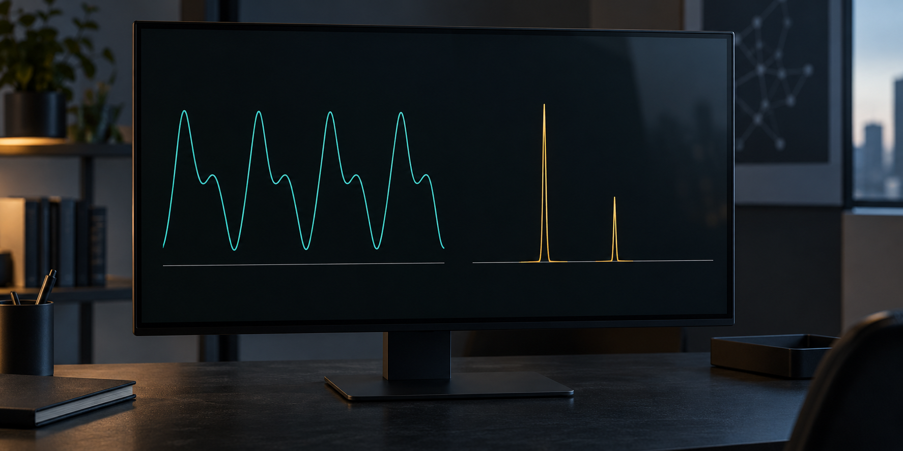
Cover: AI-generated conceptual illustration of a synthetic signal and its frequency components. It depicts neither the original computer nor experimental data.
Hearing the components inside a signal
Imagine recording a musical chord. The microphone gives you a sequence of amplitudes, while your question concerns the notes inside it. Fourier analysis provides a mathematical connection between these descriptions. Similar questions arise when studying vibrations or patterns in an image.
The discrete Fourier transform, or DFT, takes a finite sequence and expresses it through discrete frequency components. A fast Fourier transform, or FFT, is an efficient way to calculate that same transform. It is not a new kind of spectrum. NumPy's technical documentation describes the input as a time-domain signal and the output as its frequency-domain representation. DFT documentation
The practical difficulty is repetition. A direct calculation combines every input point with every output frequency. Double the number of points and the leading arithmetic work becomes four times as large. If your scientific question needs thousands of points, a mathematically simple formula can therefore become a computational obstacle.
Cooley and Tukey presented a general factorization and a convenient power-of-two implementation, including a way to reuse the input array's storage. Their paper reports an IBM 7094 program and timings, rather than only an abstract proposal. The manuscript was received on 17 August 1964 and appeared in the April 1965 issue of Mathematics of Computation. The publication day is not established here. Original paper, university copy
A breakthrough with a long prehistory
The idea did not begin from nothing in 1965. Historical researchers Michael Heideman, Don Johnson and Sidney Burrus examined earlier texts and identified an equivalent decomposition in Gauss's work. They inferred a composition date around 1805; the manuscript itself was not explicitly dated and was published posthumously in 1866. Their study also discusses later methods, including Danielson and Lanczos's 1942 work and Good's prime-factor approach. Good's restrictions differ from the general Cooley–Tukey factorization. Historical investigation and accessible author copy
In their 1993 recollection, Cooley and Tukey describe Richard Garwin's role in connecting the work and encouraging its development. They also acknowledge earlier discoveries and explain why large electronic calculations made the approach valuable. This is a retrospective account by participants, with the limits of recollection. Cooley and Tukey's account
The durable turning point was a reusable computation spreading into practice. Princeton's account of the IEEE milestone connects it with scientific computing, signal processing, medical imaging and data transmission. These applications also depend on instruments, physical models and other algorithms; the FFT contributed a powerful computational building block. The later recognition supports historical importance, rather than making a recent commemoration the discovery date. Princeton and the IEEE milestone
Four points: see the reuse before the general formula
Use the dimensionless sequence [1, 2, 3, 4]. This deliberately small example is our educational calculation, not data from the 1965 paper. Let i mean the imaginary unit, with i² = −1. The unscaled, negative-exponent DFT gives four outputs:
| Frequency index | Output |
|---|---|
| 0 | 10 |
| 1 | −2 + 2i |
| 2 | −2 |
| 3 | −2 − 2i |
The first output adds all four inputs. The others combine positive, negative and imaginary weights. A complex output records two components; its magnitude and phase describe a frequency component together.
Now separate the even-indexed inputs [1, 3] from the odd-indexed inputs [2, 4]. Each pair needs only its sum and difference:
- Even pair: E = [4, −2].
- Odd pair: O = [6, −2].
Combine those shorter results. The first butterfly produces 4 + 6 = 10 and 4 − 6 = −2. The second first rotates the odd result by −i, giving (−i)(−2) = 2i. Its two outputs are −2 + 2i and −2 − 2i.
A butterfly is the name for this paired sum-and-difference operation. Its crossing lines are bookkeeping, not a physical connection between waves. Both outputs reuse the same intermediate results. At a larger size, each shorter transform can be split again: reuse becomes a hierarchy rather than a one-off shortcut.
From the example to the scaling
For N input values, define our convention by
Xk=n=0∑N−1xne−2πink/N.
Here n indexes inputs, k indexes outputs, and both range from zero to N − 1. The factors are complex rotations of unit magnitude. Our forward transform has no normalization factor; an inverse uses the positive exponent and a factor 1/N. Other conventions exist. The original paper starts from a positive-exponent Fourier sum, so signs and normalization must be compared explicitly. Modern convention
For even N, split the sum into even and odd input indices. Write their length-N/2 transforms as Eₖ and Oₖ, and set W_N = exp(−2πi/N). For 0 ≤ k < N/2, the reconstruction is
Xk=Ek+WNkOk,Xk+N/2=Ek−WNkOk.
The second equality uses the sign change of the rotation halfway around the circle. We therefore calculate two shorter transforms and do a number of combinations proportional to N. Repeating the split for N = 2ᵐ gives m = log₂N levels.
Each level involves a quantity of work proportional to the sequence length. Consequently, the total grows as N log₂N. The notation O(N log N) describes this growth, not an exact count of processor instructions or seconds. A classroom radix-2 construction is restricted to powers of two; general Cooley–Tukey factorizations can use other composite lengths.
Speed on a real computer also depends on layout, transfers through memory and the implementation. A smaller arithmetic count alone does not establish a particular wall-clock improvement on your device.
What faster calculation cannot fix
If equally spaced measurements have interval Δt seconds, the sample rate is 1/Δt hertz and the frequency-bin spacing is 1/(NΔt) hertz. Interpreting the upper output indices requires the chosen positive/negative frequency ordering. Frequency conventions
Finite sampling still limits what can be inferred. Here t is time in seconds, f the signal frequency in hertz, and fₛ = 1/Δt the sample rate in hertz. For example, samples of cos(2πft) at t = n/fₛ are unchanged if f is replaced by f + fₛ: the added phase is 2πn. No faster algorithm can distinguish those two signals from those samples alone. Noise and inadequate measurement models likewise remain measurement problems.
Numerical arithmetic introduces another limit. Complex rotation factors generally require numerical approximations, and reordering operations can change rounding. FFTW's accuracy discussion emphasizes the importance of accurate rotation factors and documents differences between implementations and environments. Mathematical equivalence does not promise identical floating-point bit patterns. Accuracy discussion
Check the educational calculation
Our check used CPython 3.12.10 and the standard library only. The four-point roots [1, −i, −1, i] are represented exactly, so exact equality is appropriate for these small integer inputs. That criterion must not be transferred mechanically to longer floating-point transforms.
The following core calculations were executed in our recorded check:
ROOTS = (1, -1j, -1, 1j)

def direct(x, roots=ROOTS):
    return [
        sum(x[n] * roots[(n*k) % 4] for n in range(4))
        for k in range(4)
    ]

def butterfly(x):
    even = (x[0] + x[2], x[0] - x[2])
    odd = (x[1] + x[3], x[1] - x[3])
    return [
        even[0] + odd[0], even[1] - 1j*odd[1],
        even[0] - odd[0], even[1] + 1j*odd[1],
    ]
Compare both functions on [1, 2, 3, 4], an impulse [1, 0, 0, 0], a constant [1, 1, 1, 1], zeros, and [1+i, −2, 3−i, 2i]. All five agreed exactly. The first also matched the table above. Reversing the roots' imaginary signs changed the asymmetric case's spectrum, and the check rejected it as a different convention.
This validates the fixed educational cases. It neither proves every implementation correct nor independently replicates the historical performance. The original article does not supply the full program, benchmark inputs or complete timing conditions needed for such a reproduction.
Article written and translated by an AI system from the cited sources, with automated checks according to the News editorial method. The educational calculation was executed as described; it is not peer review, human scientific validation or reproduction of the historical program.